Example: Predicting Incident Rates with the Poisson Distribution

A prime example of the utility of probability distributions in public safety is the use of the Poisson distribution to predict crime rates. The Poisson distribution is particularly suited for modeling the number of times an event occurs within a fixed interval of time or space, assuming these events happen with a known constant mean rate and independently of the time since the last event.

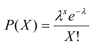
In this equation:

• P(X) is the probability "P()" that of an event occurring at the interval of "X" 
• λ (lambda) is the mean or average of the total events over a period of time
• "e" is Euler's constant which is approximately 2.178.
• X! is the product of positive integers less than or equal to X

Scenario: Modeling Burglary Rates

Consider a scenario where historical data indicates an average of two burglaries per week in a neighborhood. Public safety analysts can employ the Poisson distribution to estimate the probability of observing different numbers of burglaries in future weeks. This predictive capability is invaluable for planning and implementing proactive public safety measures.

Python Code for Predictive Analysis

To illustrate, the following Python code uses the Poisson distribution to simulate and visualize the expected number of burglaries in a neighborhood:

from scipy.stats import poisson
import numpy as np
import matplotlib.pyplot as plt

# Setting the average number of burglaries per week
lambda_ = 2

# Defining the range of possible burglaries
burglaries = np.arange(0, 10)

# Calculating probabilities using the Poisson distribution
probabilities = poisson.pmf(burglaries, lambda_)

# Visualizing the distribution
plt.figure(figsize=(10,6))
plt.bar(burglaries, probabilities, color='skyblue')
plt.title('Probability Distribution of Burglaries per Week')
plt.xlabel('Number of Burglaries')
plt.ylabel('Probability')
plt.show()

What is this code doing?

Define Parameters:

• lambda_ = 2: Sets the average rate (λ, lambda) of burglaries per week to 2. This is a key parameter of the Poisson distribution, representing the mean number of events (burglaries) expected to occur in a fixed interval (one week).

Create Range of Possible Burglaries:

• burglaries = np.arange(0, 10): Generates an array of integers from 0 to 9 using NumPy's arange function. This array represents the range of possible numbers of burglaries that the analysis will consider.

Calculate Probabilities:

• probabilities = poisson.pmf(burglaries, lambda_): Calculates the probability mass function (PMF) for each value in the burglaries array given the average rate lambda_. The PMF returns the probability of a given number of events (here, burglaries) occurring in a fixed interval, based on the Poisson distribution.

Visualize the Distribution:

The code then creates a bar chart to visualize the probabilities calculated for each number of burglaries.

• plt.figure(figsize=(10,6)): Creates a new figure with a specified size (10 inches by 6 inches) for the plot.
• plt.bar(burglaries, probabilities, color='skyblue'): Plots a bar chart where the x-axis represents the number of burglaries (from 0 to 9) and the y-axis represents their corresponding probabilities. The bars are colored sky blue.
• plt.title(...), plt.xlabel(...), plt.ylabel(...): These commands add a title to the chart and labels to the x-axis and y-axis, respectively, enhancing the readability of the plot.
• plt.show(): Displays the plot. This visualization helps in understanding the distribution of probabilities for the number of burglaries, highlighting how likely each outcome is within the given week, based on the Poisson distribution.

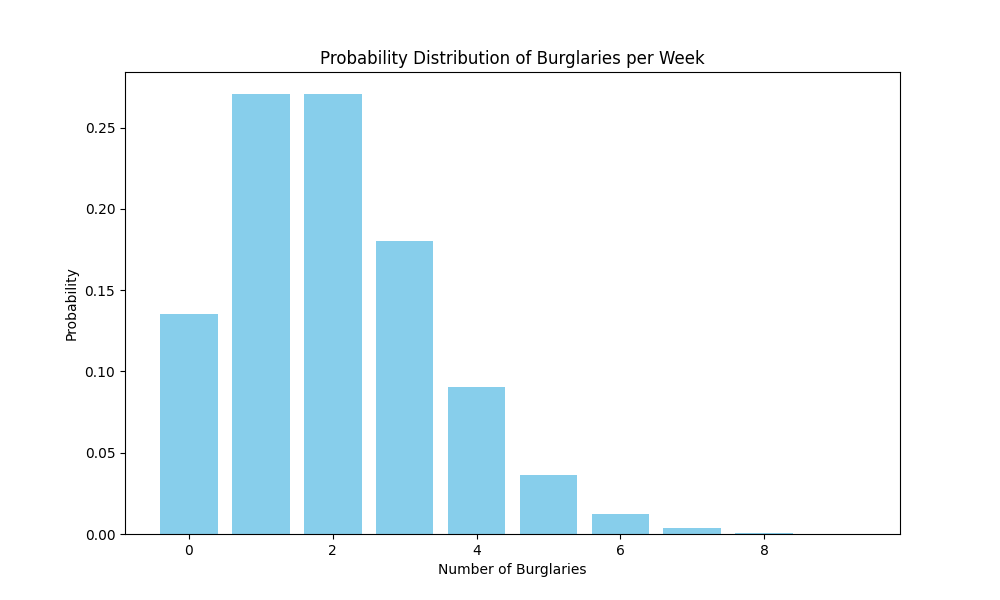
This visualization effectively communicates the likelihood of various burglary counts, aiding analysts in understanding and communicating the risk levels to decision-makers and the public.

The Role of Predictive Analysis in Public Safety

Predictive analysis, powered by probability distributions, plays a critical role in public safety. By estimating the likelihood of future incidents, public safety officials can better allocate resources, enhance surveillance, and implement preventive measures. For instance, a higher predicted rate of burglaries might prompt increased patrols or community awareness programs during periods of elevated risk.

Moreover, this analytical approach supports a shift from reactive to proactive public safety strategies. It enables authorities to anticipate and mitigate risks before they escalate, thus contributing to safer communities.

Conclusion

Probability distributions are powerful tools that significantly enhance the predictive capabilities of public safety intelligence analysts. By enabling accurate forecasting of crime rates and other incidents, they facilitate informed decision-making and proactive public safety measures. As we continue to explore statistical methods and their applications in public safety, the value of predictive analysis in fostering secure and resilient communities becomes increasingly clear.