Example: Crime Rate Analysis

Consider an analysis of crime rates across various districts within a city. Descriptive statistics can reveal the average crime rate (mean), the district with the median crime rate, and the most common type of crime (mode). Variability measures, such as the standard deviation, can indicate how much crime rates differ from one district to another, offering insights into areas with higher variability in crime rates and potentially identifying areas requiring focused interventions.

Understanding these statistics allows public safety officials to allocate resources more effectively, targeting areas with higher crime rates or greater variability in crime types. This can lead to more strategic policing and community safety initiatives.

We can create a dataset representing the crime rates per 100,000 inhabitants in different districts and use descriptive statistics to summarize this data.

import pandas as pd
import numpy as np
import matplotlib.pyplot as plt
import seaborn as sns

# Sample data: Crime rates per 100,000 inhabitants in different districts
data = {'District': ['District A', 'District B', 'District C', 'District D', 'District E'],
        'Crime Rate': [450, 300, 500, 250, 400]}
df = pd.DataFrame(data)

# Descriptive statistics
mean_crime_rate = df['Crime Rate'].mean()
median_crime_rate = df['Crime Rate'].median()
mode_crime_rate = df['Crime Rate'].mode()[0]
std_deviation = df['Crime Rate'].std()

print(f"Mean Crime Rate: {mean_crime_rate}")
print(f"Median Crime Rate: {median_crime_rate}")
print(f"Mode Crime Rate: {mode_crime_rate}")
print(f"Standard Deviation: {std_deviation}")

# Plot
plt.figure(figsize=(10,6))
sns.barplot(x='District', y='Crime Rate', hue='District', data=df, palette='coolwarm', legend=False)
plt.title('Crime Rate by District')
plt.show()

First, we will look at what is output from this code snippet, then we will dive into what it all means and how it can be utilized.

Output:

Mean Crime Rate: 380.0
Median Crime Rate: 400.0
Mode Crime Rate: 250
Standard Deviation: 103.6822067666386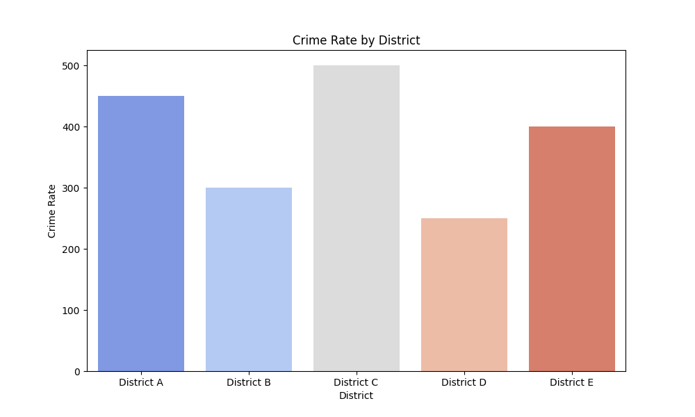

This Python code snippet demonstrates how to perform basic descriptive statistical analysis and visualization on crime rate data across various districts. It utilizes libraries such as pandas for data manipulation, numpy for numerical calculations, and matplotlib and seaborn for data visualization. Here's a step-by-step breakdown of its components and their significance for intelligence analysts:

1. Data Creation: The code begins by creating a dataset with pandas DataFrame, which includes the crime rates per 100,000 inhabitants for five different districts (labeled District A to District E). This dataset serves as a simplified model for understanding crime distribution in a city or region.

2. Descriptive Statistics Calculation:

   • Mean Crime Rate: Calculates the average crime rate across all districts, providing a general idea of the overall crime level.
   • Median Crime Rate: Identifies the middle value of the crime rates when they are ordered from lowest to highest, offering insight into the central tendency of the data without being skewed by outliers.
   • Mode Crime Rate: Finds the most frequently occurring crime rate among the districts, which could be useful for identifying common crime levels or patterns.
   • Standard Deviation: Measures the amount of variation or dispersion of crime rates from the mean, indicating how spread out the crime rates are across districts. A higher standard deviation suggests more variability in crime rates.

3. Data Visualization:

   • The code then plots a bar chart using seaborn, with districts on the x-axis and their respective crime rates on the y-axis. This visual representation makes it easier to compare crime rates across districts at a glance, highlighting areas of higher or lower safety.

How Can This Be Used By Analysts?

• Trend Analysis: By examining the mean, median, and mode, analysts can assess overall crime trends and identify typical crime levels, aiding in the development of long-term public safety strategies.
• Understanding Variability: The standard deviation helps analysts understand the uniformity of crime rates across districts. Districts with high variability might have underlying issues that require further investigation.

Conclusion

This analysis of descriptive statistics illuminates how critical data-driven insights are in shaping public safety strategies. Through the calculation of mean, median, mode, and standard deviation, we uncover not just the average crime rates but also their distribution across districts, guiding the effective allocation of resources and targeted interventions. The visual comparison further enhances our understanding, pinpointing areas in need of attention.

Transitioning from this foundational groundwork, our next focus will be on Probability Distributions. This segment will elevate our analytical prowess by equipping us with forecasting tools essential for anticipating crime trends and preparing proactive measures. Such predictive analytics are vital for optimizing public safety efforts, ensuring resources are utilized where they're most needed to foster safer communities. Join us as we delve deeper into these methods, exploring their application in the realm of public safety intelligence analysis.